Contents
- 第三章 matlab绘图
- 一.二维数据曲线的绘制
- 1.单独二维曲线的绘制
- 2.多根二维曲线的绘制
- 1)plot函数的输入参数是矩阵形式
- 2)含多个输入参数的plot的函数
- 3)plotyy函数[AX,H1,H2] = plotyy(x1,y2,x2,y2,'function')
- 3.设置曲线样式 | 颜色,线型,标记符号.
- 4.图形的标注与坐标控制
- 1)图形的标注
- 2)坐标控制
- 5.图形窗口的分割
- 二.其他二维图形的绘制
- 1.特殊坐标图形
- 1)绘制对数坐标图形
- 2)绘制极坐标图形
- 2.特殊二维图形的绘制
- 1)条形图的绘制 bar
- 2)面积图的绘制area
- 3)饼图的绘制pie pie3
- 4)火柴杆图的绘制stem
- 5)矢量图的绘制
- 6)绘制等高线contour
- 为了节约内存,这里运行完成程序后清空.
第三章 matlab绘图
clc;
clear all;
close all;
一.二维数据曲线的绘制
1.单独二维曲线的绘制
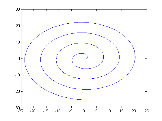
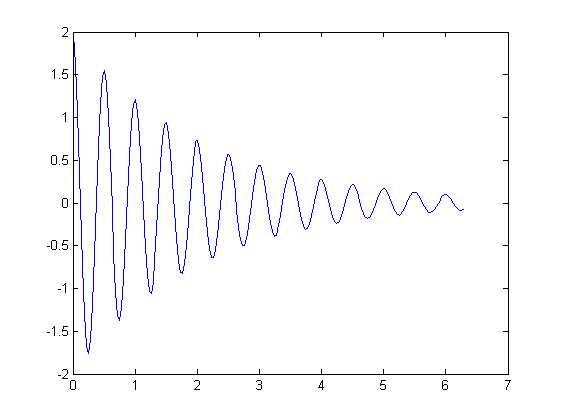
% plot(x,y)

% % 在0<=x<=2*pi区间内,绘制曲线y=2*exp(-0.5*x)*cos(4*pi*x)
 x = 0:pi/100:2*pi;
 y =2*exp(-0.5*x).*cos(4*pi*x);
 figure;
 plot(x,y)

% % 绘制曲线x = cost+tsint  y = sint -tcost
t = 0:0.1:8*pi;
x = cos(t)+t.*sin(t);
y = sin(t)-t.*cos(t);
figure
plot(x,y)
2.多根二维曲线的绘制
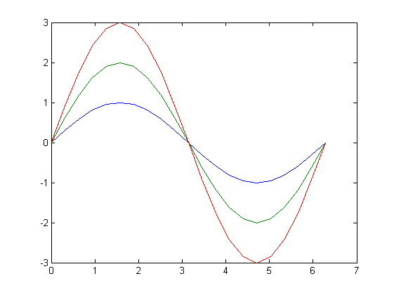
1)plot函数的输入参数是矩阵形式
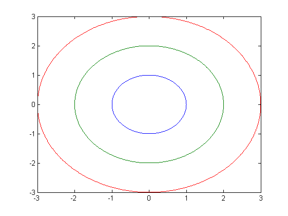
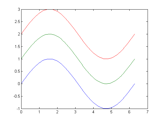
% % 当x是向量时,y是也有一维与x同维的矩阵时.
x = linspace(0,2*pi,100);
y =[sin(x);1+sin(x);2+sin(x)];
figure
plot(x,y)

% %x,y是同维矩阵.
x = 0:pi/10:2*pi;
y = sin(x);
figure
plot([x;x;x]',[y;y*2;y*3]')

% %当输入参数是实矩阵时,则按列绘制没列元素值相对于其坐标下的曲线.
t = 0:0.01:2*pi;
x = exp(i*t);
y = [x;x*2;x*3]';
figure
plot(y)
2)含多个输入参数的plot的函数
% %当plot函数有多个输入参数,每两个组成一组.
x = 0:pi/10:2*pi;
y = sin(x);
figure
plot(x,y,x,y*2,x,y*3)
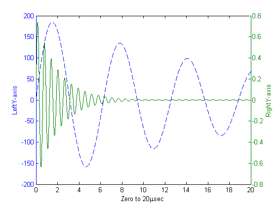
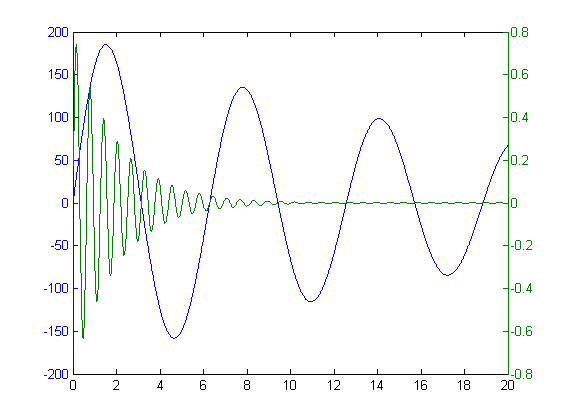
3)plotyy函数[AX,H1,H2] = plotyy(x1,y2,x2,y2,'function')
% 格式 :
% plotyy(x1,y1,x2,y2)
% plotyy(x1,y2,x2,y2,'function')
% [AX,H1,H2] = plotyy(x1,y2,x2,y2,'function')

% % 使用函数plotyy绘制两个数学函数
x = 0:0.01:20;
y1 = 200*exp(-0.05*x).*sin(x);
y2 = 0.8*exp(-0.5*x).*sin(10*x);
figure
[AX,H1,H2] = plotyy(x,y1,x,y2,'plot');

% % 添加样式x = 0:0.01:20;
y1 = 200*exp(-0.05*x).*sin(x);
y2 = 0.8*exp(-0.5*x).*sin(10*x);
figure
[AX,H1,H2] = plotyy(x,y1,x,y2,'plot');

set(get(AX(1),'Ylabel'),'String','LeftY-axis');         % AX(1)是左侧的y轴
set(get(AX(2),'Ylabel'),'String','RightY-axis');        % AX(2)是右侧的y轴
xlabel('Zero to 20\musec');                             % 添加x轴的标签
set(H1,'LineStyle','--');                               % H1所代表的曲线.
set(H2,'LineStyle','-');                                % H2所代表的曲线.
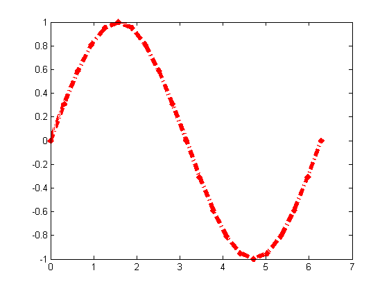
3.设置曲线样式 | 颜色,线型,标记符号.
% %--------------------
% 颜色选项          颜色
% b(blue)          蓝色
% g(green)         绿色
% r(red)           红色
% c(cyan)          青色
% m(magenta)       品红色
% y(yellow)        黄色
% b(black)         黑色
% w(white)         白色

% %--------------------
% 线型选项       线型
% -             实线
% :             虚线
% -.           点划线
% --           双划线

% %--------------------
% 选项           标记符号
% .               点
% O               圆圈
% X               叉号
% +               加号
% *               星号
% s(square)      方块符
% d(diamond)     菱形符
% v              朝下三角符号
% ^              朝上三角符号
% <              朝左三角符号
% >              朝右三角符号
% p(pentagram)   五角星符
% h(hexagram)    六角星符

% % 以线宽5,红色,点画线,叉号形式绘画x在[0,2*pi]内的正弦函数y=sin(x)的图形.
x = 0:pi/10:2*pi;
y = sin(x);
figure
plot(x,y,'r-.X','LineWidth',5);
4.图形的标注与坐标控制
1)图形的标注
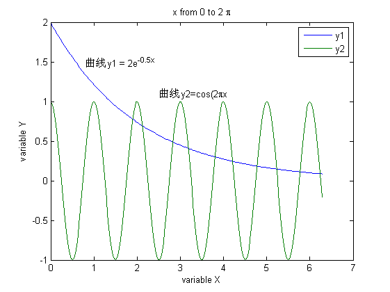
% title(s)  书写图名
% xlabel(s) 横坐标轴名
% ylabel(s) 纵坐标轴名
% legend(s1,s2) 绘制曲线的图例
% text(xt,yt,s) 在图里(xt,yt)坐标处书写字符注释.

% %---------------常用的LaTeX字符---------------------
% \alpha	α	\upsilon	υ	\sim	~
% \beta	β	\phi	?	\leq	≤
% \gamma	γ	\chi	χ	\infty	∞
% \delta	δ	\psi	ψ	\clubsuit
% \epsilon	?	\omega	ω	\diamondsuit
% \zeta	ζ	\Gamma	Γ	\heartsuit
% \eta	η	\Delta	Δ	\spadesuit
% \theta	θ	\Theta	Θ	\leftrightarrow	?
% \vartheta	?	\Lambda	Λ	\leftarrow	←
% \iota	ι	\Xi	Ξ	\uparrow	↑
% \kappa	κ	\Pi	Π	\rightarrow	→
% \lambda	λ	\Sigma	Σ	\downarrow	↓
% \mu	μ	\Upsilon	Υ	\circ	°
% \nu	ν	\Phi	Φ	\pm	±
% \xi	ξ	\Psi	Ψ	\geq	≥
% \pi	π	\Omega	Ω	\propto	∝
% \rho	ρ	\forall	?	\partial	?
% \sigma	σ	\exists	?	\bullet	?
% \varsigma	?	\ni
% \div	÷
% \tau	τ	\cong	?	\neq	≠
% \equiv	≡	\approx	≈	\aleph	?
% \Im
% \Re
% \wp
% \otimes	?	\oplus	?	\oslash
% \cap	∩	\cup	∪	\supseteq	?
% \supset	?	\subseteq	?	\subset	?
% \int	∫	\in	∈	\o	ο
% \rfloor
% \lceil
% \nabla
% \lfloor
% \cdot
% \ldots
% \perp
% \neg
% \prime
% \wedge
% \times
% \0	?
% \rceil
% \surd
% \mid	|
% \vee
% \varpi
% \copyright	?
% \langle
% \rangle

% % 在0,2pi区间,绘制曲线y1= 2exp(-0.5x)和y2=cos(2*pi*x),并给图形添加标注.

x = 0:pi/100:2*pi;
y1=2*exp(-0.5*x);
y2 = cos(2*pi*x);
figure
plot(x,y1,x,y2)
title('x from 0 to 2 {\pi}')
xlabel('variable X')
ylabel('variable Y')
text(0.8,1.5,'曲线y1 = 2e^{-0.5x}')
text(2.5,1.1,'曲线y2=cos(2{\pi}x')
legend('y1','y2')
2)坐标控制
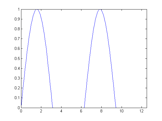
% % axis([xmin xmax ymin ymax])

% %---------------------------------------------
% % 在0,4pi区间内,画出正弦波在y轴介于0和1的部分.
x  =0:0.1:4*pi;
y = sin(x);
plot(x,y)
axis([-inf inf 0 1])

% %---------------------------------------------
% % 绘制曲线y=sintsin(7t)及其包络线.
t = (0:pi/100:pi)';
y1 = sin(t)*[1,-1];
y2 = sin(t).*sin(7*t);
figure
plot (t,[y1,y2]');
grid on
box on
axis equal
5.图形窗口的分割
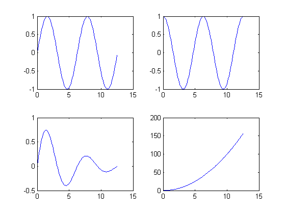
% % subplot(m,n,p)          m行n列的第p个绘图区域.


% %---------------------------------------------
% %在一个窗口中同时绘制出4个图形.
x = 0:0.1:4*pi;
subplot(2,2,1);
plot(x,sin(x))              %此为左上角图形.

subplot(2,2,2);
plot(x,cos(x))              %此为右上角图形.

subplot(2,2,3);
plot(x,sin(x).*exp(-x/5))              %此为左下角图形.

subplot(2,2,4);
plot(x,x.^2)              %此为右下角图形.
二.其他二维图形的绘制
1.特殊坐标图形
1)绘制对数坐标图形
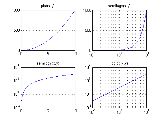
% % semilogx(x1,y1,选项1,x2,y2,选项2...)
% % semilogy(x1,y1,选项1,x2,y2,选项2...)
% %loglog(x1,y1,选项1,x2,y2,选项2...)

% %---------------------------------------------
% %绘制y=10*x*x的对数座标图形和指教线性坐标图形.

x = 0:0.1:10;
y = 10*x.*x;

figure

subplot(2,2,1)
plot(x,y)
title('plot(x,y)')
grid on

subplot(2,2,2)
semilogx(x,y);
title('semilogx(x,y)')
grid on

subplot(2,2,3)
semilogy(x,y);
title('semilogy(x,y)')
grid on

subplot(2,2,4)
loglog(x,y);
title('loglog(x,y)')
grid on
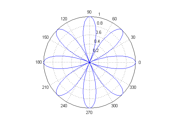
2)绘制极坐标图形
% %polar(t,r,option)
% % t角度
% % r幅度向量
% % option选项.

% %---------------------------------------------
% %绘制y=2sin(2t-pi/4)cos(2t-pi/4)的极坐标图形,并标注数据点.
t = 0:0.01:2*pi;
r = 2*sin(2*(t-pi/8)).*cos(2*(t-pi/8));
figure
polar(t,r)
2.特殊二维图形的绘制
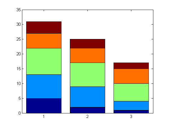
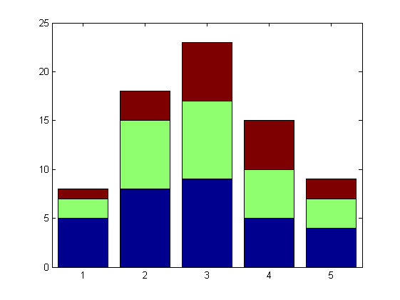
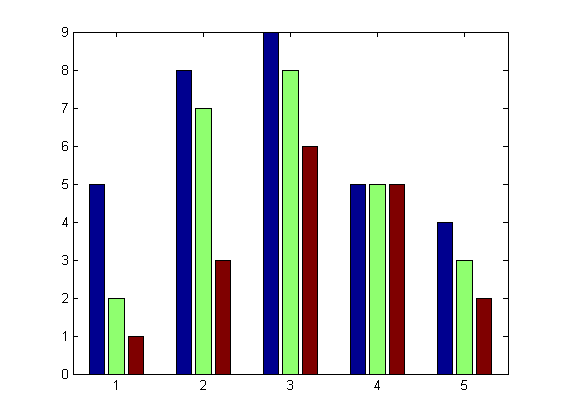
1)条形图的绘制 bar
%  bar(y,option)              以x=1,2,3...为x坐标,y的对应元素为y坐标画垂直放置的二维条形图
%  bar(x,y,option)            以x各个元素为x坐标,y的对应元素为y坐标画垂直放置的二维条形图
%  bar(y,'stack')             以x=1,2,3...为x坐标,y的各[行]元素为累加值为y坐标.
%  bar(y,'group')             以x=1,2,3...为x坐标,y的各[列]元素的累加值为y坐标.

% %---------------------------------------------
% %用给定的数据绘制二维条形图
Y=[5 2 1;8 7 3; 9 8 6;5 5 5 ;4 3 2];
bar(Y)
figure
bar(Y,'stack')
figure
bar(Y,'group')                %似乎group不对头....
figure
bar(Y','stack')
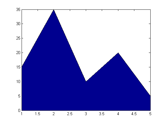
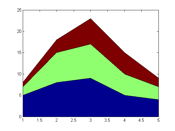
2)面积图的绘制area
% %area(y)               以x=1,2,3...为x坐标,y的对应元素为y坐标画二维折线图,并填充与x轴的区域.
% %area(x,y)             以x各个元素为x坐标,y的对应元素为y坐标画二维折线图,并填充与x轴的区域.
y = [15,35,10,20,5];
area(y)
Y=[5 2 1;8 7 3; 9 8 6;5 5 5 ;4 3 2];
figure
area(Y)                  %以Y的每一列y为一组值画图.
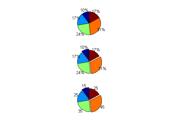
3)饼图的绘制pie pie3
% %pie(y) 绘制每一元素占全部向量元素的总和值的百分比.
% %pie(y,explode) explode为与y同维的0,1向量,非0表示对应y元素从饼图中分离出来.
% % pie3 绘制3维饼图.
y = [ 15 25 35 45 25 ]
figure
subplot(3,1,1)
pie(y)
subplot(3,1,2)
pie(y,[1 0 0 1 0 ])
subplot(3,1,3)
pie(y,[1 0 0 1 0 ],{'15','25','35','45','25'})
y =

    15    25    35    45    25
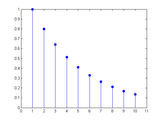
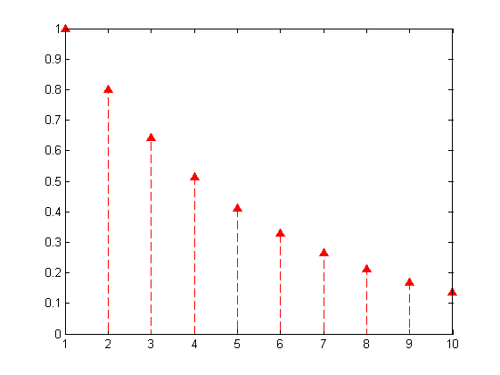
4)火柴杆图的绘制stem
% %stem(y)
% %stem(x,y,option)
% %stem(x,y,'filled')

% %---------------------------------------------
y = linspace(0,2,10)
figure
stem(exp(-y),'filled')
axis([0 11 0 1])
figure
stem(exp(-y),'filled','r--^')  % 实际使用的是 stem(y,'filled',option)
    % 其中option为线型,线颜色,点型,点颜色.
y =

         0    0.2222    0.4444    0.6667    0.8889    1.1111    1.3333    1.5556    1.7778    2.0000
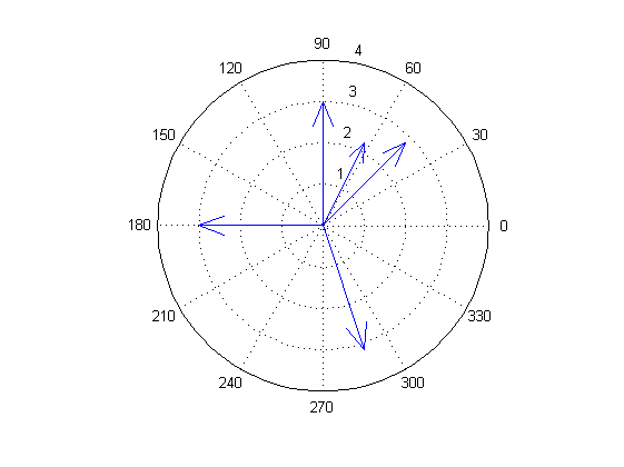
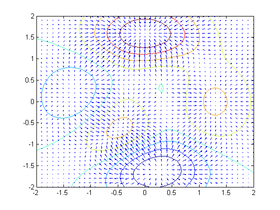
5)矢量图的绘制
% compass 绘制从源极点散发的矢量
% feather 从一个水平直线等间距出发,图形显示矢量.
% quiver 显示2D矢量场.

% %---------------------------------------------
z = [1+2j 2+2j 1-3j 3j -3]
figure
compass(z)
figure
feather(z)
grid on

% %---------------------------------------------
% % 【预备知识】
% %  FX = gradient(F)
%   其中F是一个向量。该格式返回F的一维数值梯度。FX即?F/?x,即沿着x轴(水平轴)方向的导数。
%   [FX,FY] = gradient(F)
%   其中F是一个矩阵。该调用返回二维数值梯度的x、y部分。FX对应?F/?x, FY对应于?F/?y。
%   [FX,FY,FZ,...] = gradient(F)
%   这里,F是一个含有N个自变量的多元函数。
%   [...] = gradient(F,h)
%   这里的h指定了沿着梯度的方向取点的间隔。
%   [...] = gradient(F,h1,h2,...)

% %   contour(X,Y,Z), contour(X,Y,Z,n), and contour(X,Y,Z,v) draw contour plots
%   of Z使用Z来画等高线
%    using X and Y to determine the x- and y-axis limits. X和Y用来定X,Y的限制.
%   When X and Y are matrices,
%   they must be the same size as Z and must be monotonically increasing.
% % 【预备知识】


%  %  [X,Y,Z] = peaks(n);   %返回Z为高斯分布的离散值.X,Y为画三维曲线在xoy平面的投影区域

% % 使用quiver命令画一个矢量场
n= -2.0:0.1:2.0;
[X,Y,Z] = peaks(n);             %返回Z为高斯分布的离散值.X,Y为画三维曲线在xoy平面的投影区域
contour(X,Y,Z,8);               %1.绘制等高线,等高线分8条等高.
hold on
[Zx,Zy]= gradient(Z,0.2);       %平均0.2间隔采样曲面Z,然后求点处的梯度.
quiver(X,Y,Zx,Zy);              %2.在点(x,y)处绘制向量(Zx,Zy)
hold off
z =

   1.0000 + 2.0000i   2.0000 + 2.0000i   1.0000 - 3.0000i        0 + 3.0000i  -3.0000
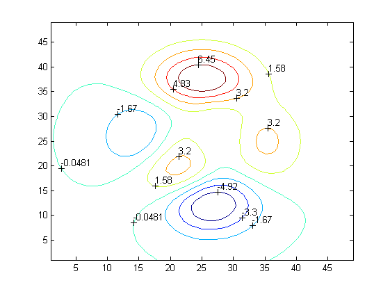
6)绘制等高线contour
% contour(Z)    绘制矩阵Z的等值线图.
% contour(Z,n)  绘制n个等值水平的Z矩阵的等值线图
% c=contourc(Z,n) 计算等高线的坐标
% clable(c)     给等高线加标注.

% %-----------------------------------
% % 在二维平面上绘制peaks函数的8条等高线.
contour(peaks,8)            %绘制peaks函数的8条等高线
c = contourc(peaks,8);      %计算等高线坐标
clabel(c)                   %添加等高线标注.
% n= -2.0:0.1:2.0;
% Z = peaks(n);
% contour(Z,8)
% c = contourc(peaks,8);
% clabel(c)